Multilevel Modeing (with R)
Princeton University
4/24/23
Overview
What are multilevel models and why are they awesome?
Important terminology
Interpretation, estimation, and visualization of multilevel models in R
Writing up MLM results
What we wont have time to talk about 😿
Cross-classified models
Partial-pooling/shrinkage
Growth curve modeling
Different types of degrees of freedom
Centering
Effective sample size
Power
Cross-level interactions
If you have specific questions about these things ask me
Why multilevel modeling?
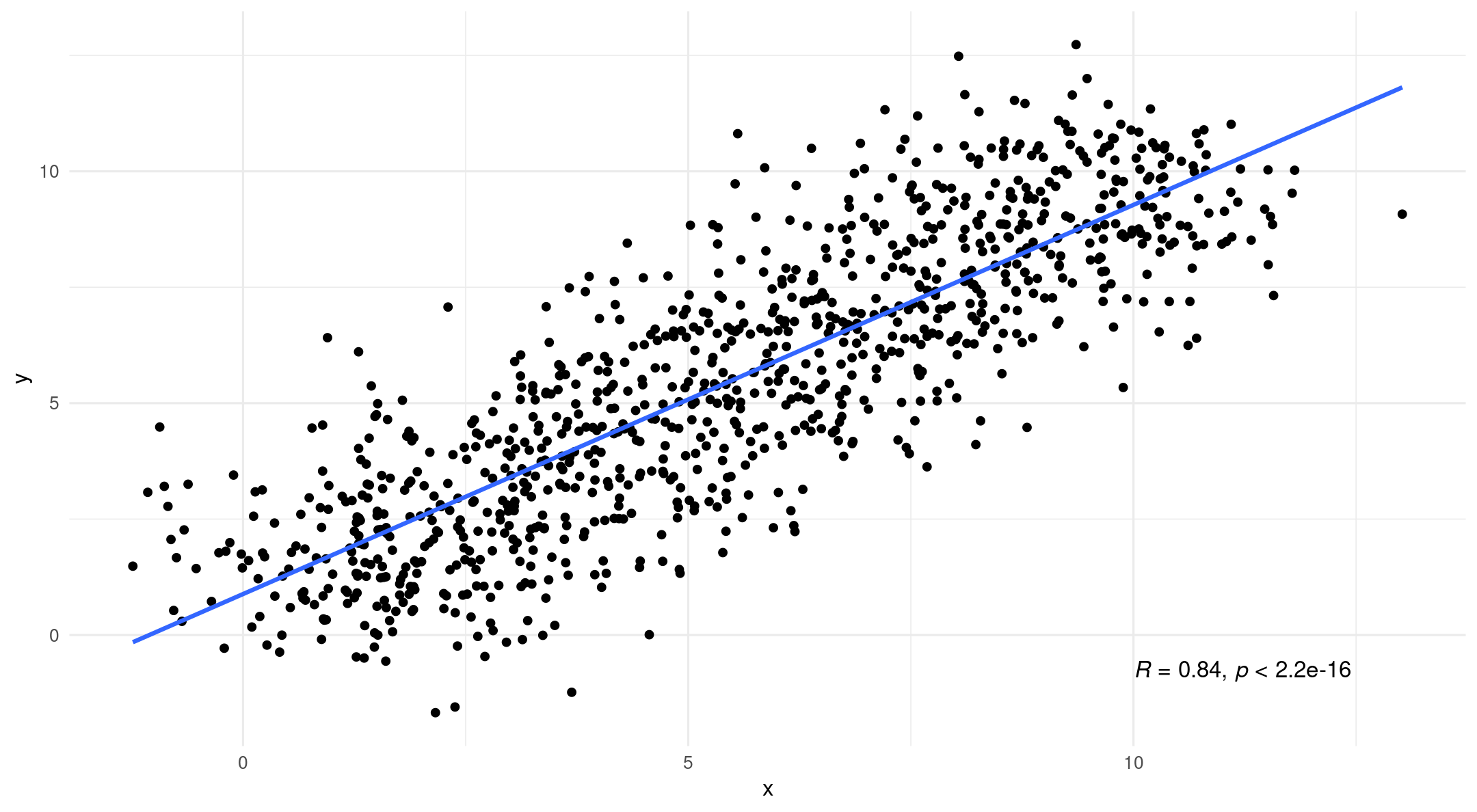
You might be used to your data looking like this: An independent variable (x) and a dependent variable (y)
![]()
Why multilevel modeling?
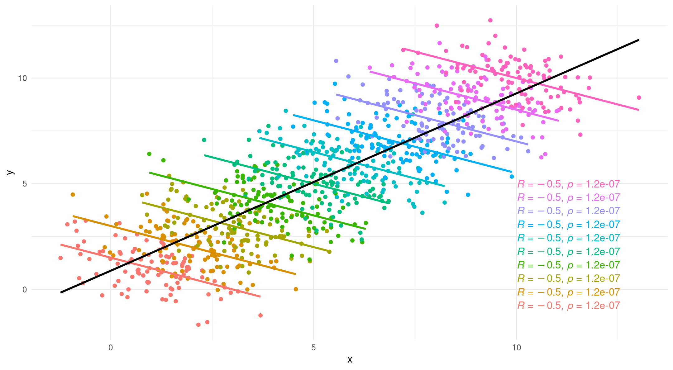
- However, if we introduce grouping we tell a different story
What is multilevel modeling?
- Simpson’s Paradox

What is multilevel modeling?
What is multilevel modeling?
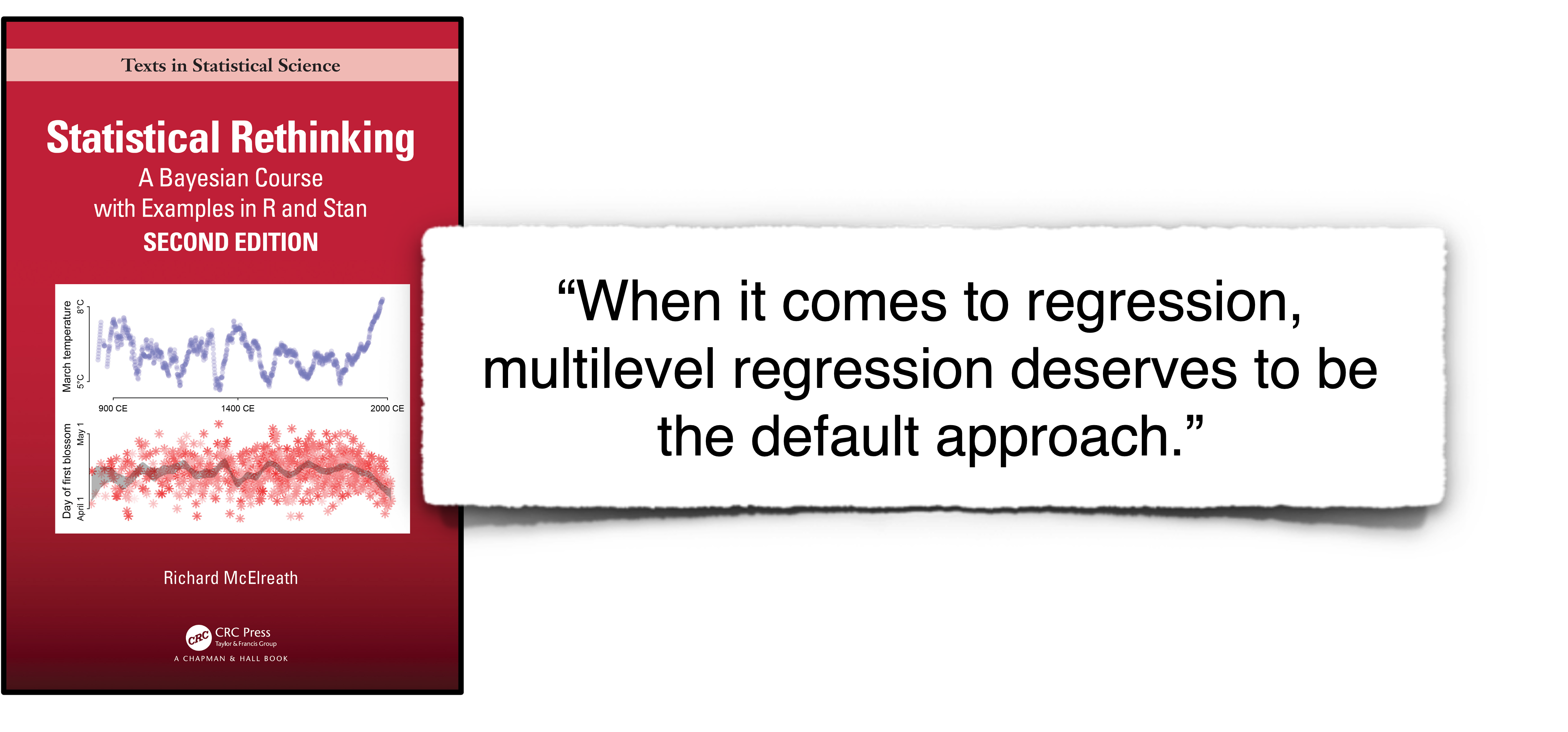
- An elaboration on regression to deal with non-independence between data points (i.e., clustered data)
Hierarchies

- For now we will focus on data with two levels:
- Level one: most basic level of observation
- Level two: groups formed from aggregated level-one observation
Multilevel models are awesome!
- Interdependence
- You can model the relationships between cases (regression for repeated observations)
- Missing data
- Uses ML for missing data (partial pooling or shrinkage)
- Power
- Deaggregated data
- Take into account within and between variance
- Flexibility

Multilevel models
When to use them:
Nested designs
Repeated measures
Longitudinal data
Why use them:
- Captures variance occurring between groups and within groups
What they are:
- Linear model with extra residuals
Important Terminology
Jumping right in
Words you hear constantly in MLM Land:
- Fixed effects
- Random effects
- Random intercepts
- Random slopes
What do they all mean?
Today’s data
What did you say?
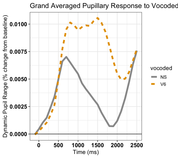
- Ps (N = 31) listened to clear (NS) and 6 channel vocoded speech (V6)
- (https://www.mrc-cbu.cam.ac.uk/personal/matt.davis/vocode/a1_6.wav)
- Ps (N = 31) listened to clear (NS) and 6 channel vocoded speech (V6)
Data
library(tidyverse)
library(lme4) # fit mixed models
library(broom.mixed) # tidy output of mixed models
library(afex) # fit mixed models
library(emmeans) # marginal means
library(ggeffects) # marginal means
eye  <- read_csv("https://raw.githubusercontent.com/jgeller112/psy504-advanced-stats/main/slides/MLM/data/vocoded_pupil.csv")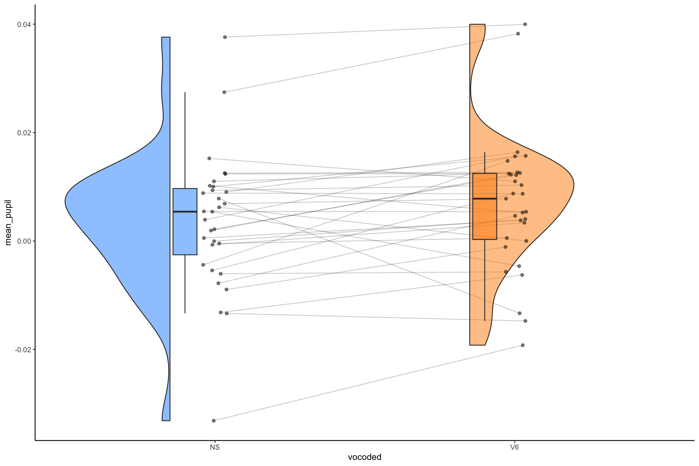
Fixed and random effects
Fixed effect:
Assumed to be constant
Population-level (i.e., average) effects that should persist across experiments
Usually experimental manipulations
Can be continuous or categorical
In our data:
vocoded
Fixed and random effects
Random effects:
Assumed to vary at the group/cluster-level
Randomly sampled observations over which you plan to generalize
- Participants
- Schools
- Words
- Pictures
Can help account for individual variation
In our data:
subject
Random intercepts
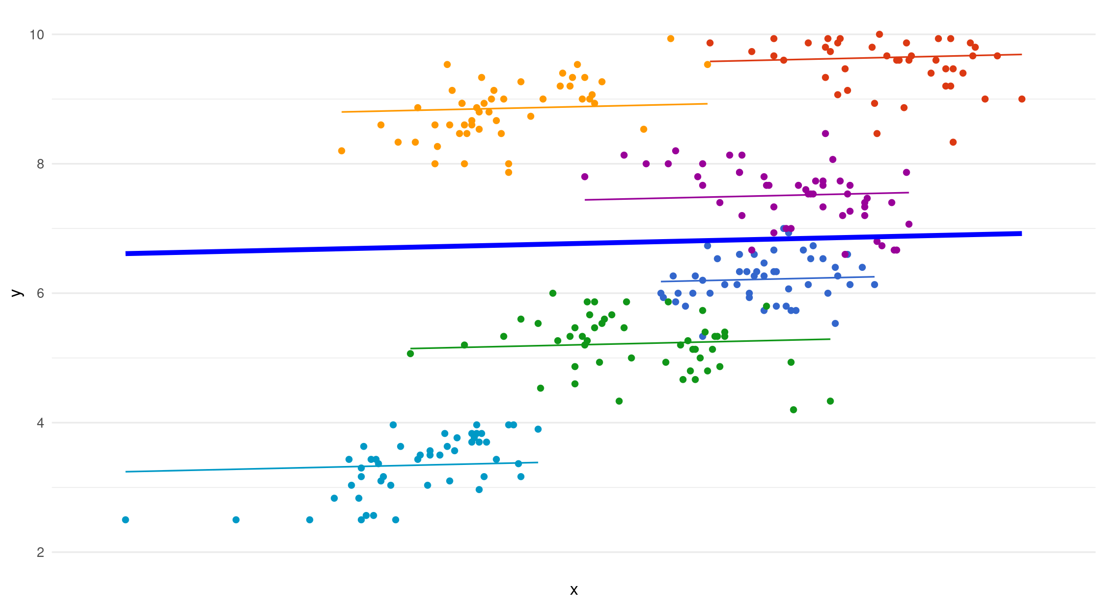
Varying starting point (intercept), same slope for each group
(1|participant): random intercept for group
Random intercepts
In a multilevel model, error terms for individual data points are estimated by group
Person-specific deviation from group’s predicted outcome
\[ y_{ij} = (\beta_{0} + u_{0j}) \]
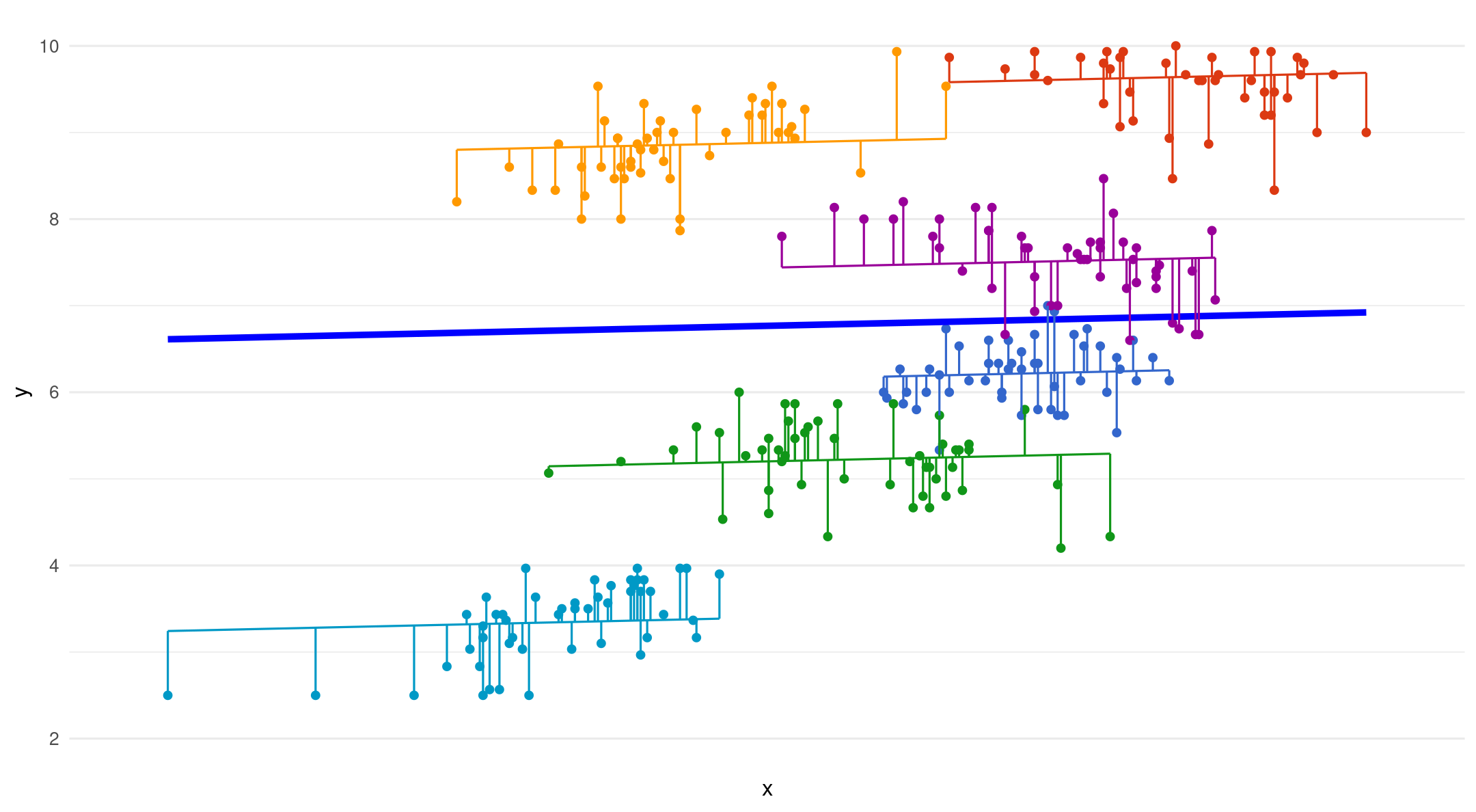
Random intercepts - fixed slopes
Random intercepts - random slopes
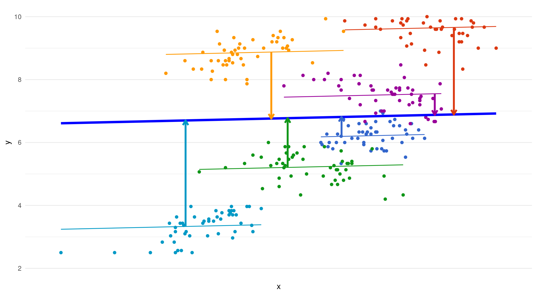
Varying starting point (intercept) and slope per group
(1+vocoded|group): random intercept and slopes per group
Only put a random slope if it changes within cluster/group
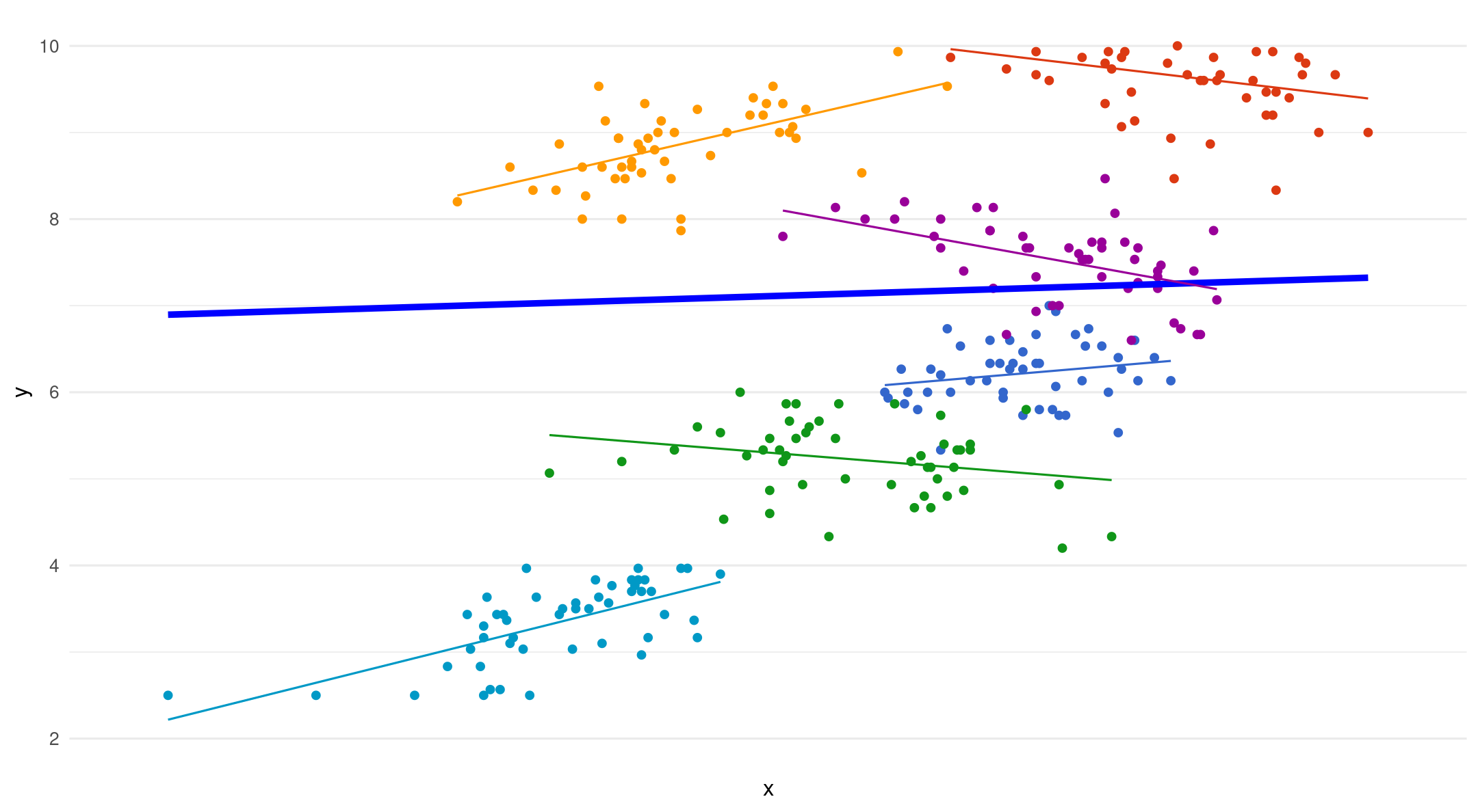
Random intercepts - random slope
- The dotted lines are fixed slopes. The arrows show the added error term for each random slope
\[ y_{ij}=(\beta_{1} + u_{1j}) \]
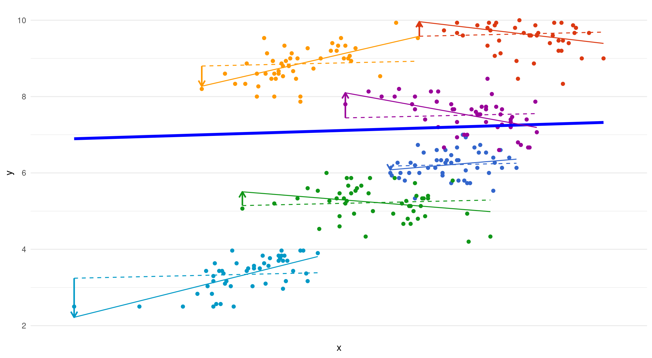
All together
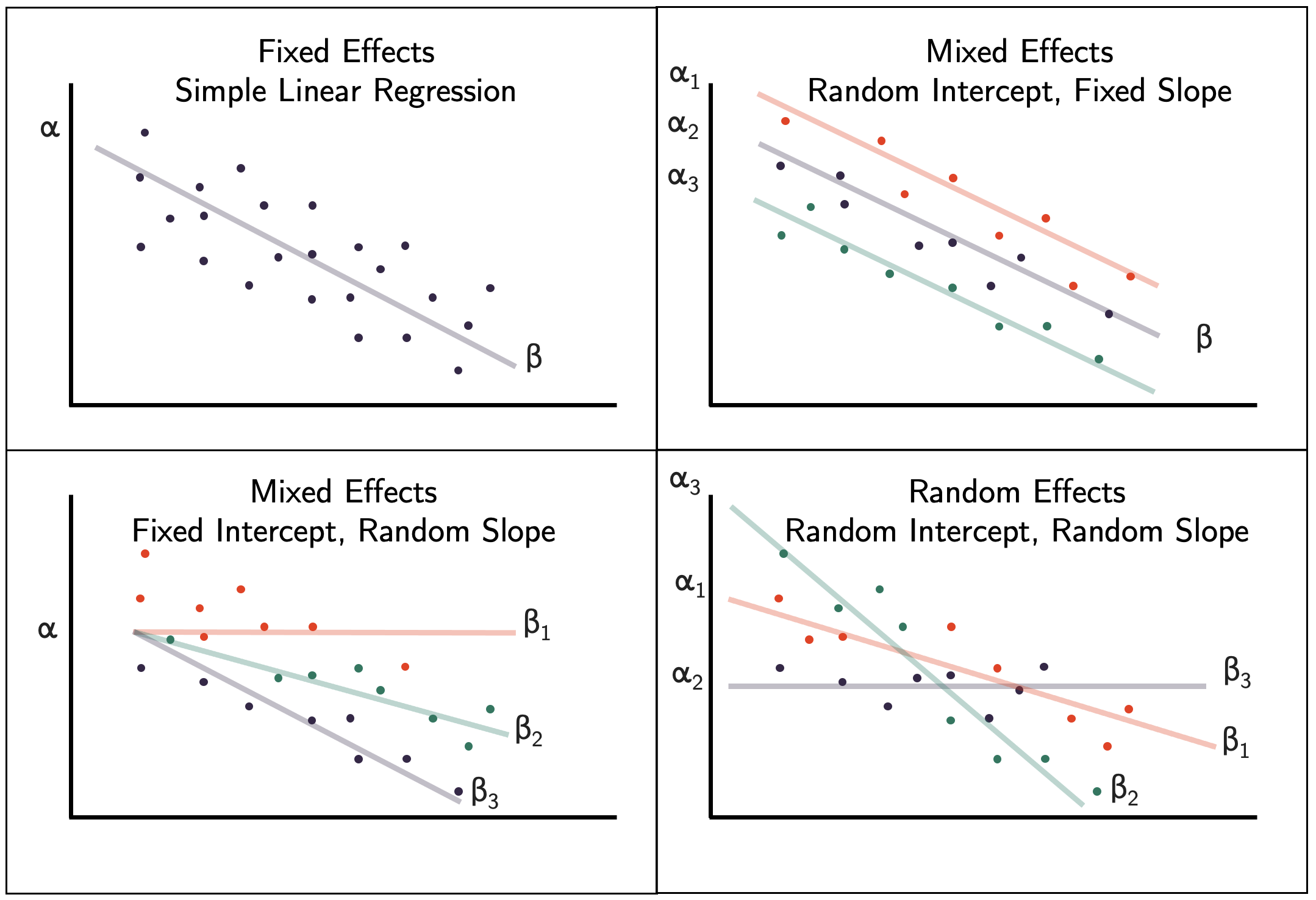
Combined multilevel equation
- Level 1: \[y_{ij} = \beta_{0j} + \beta_{1j}x_{ij} + e_{ij}\]
- Level 2:
\[ Random Intercept = \beta_{0j} = \beta_{0} + u_{0j}\]
\[Random{slope}=\beta_{1j} = \beta_{1} + u_{1j}\]
- Mixed Model Equation
\[y_{ij} = (\beta_{0} + u_{0j}) + (\beta_{1} + u_{1j})x_{ij} + e_{ij}\]
Modeling
Data organization
Data Structure
- MLM analysis requires data in long format
| ...1 | subject | trial | vocoded | mean_pupil |
|---|---|---|---|---|
| 1 | EYE15 | 3 | V6 | 0.084 |
| 2 | EYE15 | 4 | V6 | 0.0141 |
| 3 | EYE15 | 5 | V6 | 0.0225 |
| 4 | EYE15 | 6 | V6 | 0.000742 |
| 5 | EYE15 | 7 | V6 | 0.0243 |
| 6 | EYE15 | 8 | V6 | 0.0268 |
Model selection
Forward or backward approach
Model 1: Null (unconditional means) model (calculate ICC)
Model 2: full (maximal) model
if non-convergence (pay attention to warning messages):
Try different optimizers 1
Deal with random effects
Model 3 (optional): remove fixed effects (e.g., interaction)
Model fitting: ML or REML
Two flavors of maximum likelihood
Maximum Likelihood (ML or FIML)
Jointly estimate the fixed effects and variance components using all the sample data
Can be used to draw conclusions about fixed and random effects
Issue: Fixed effects are treated as known values when estimating variance components
- Results in biased estimates of variance components (especially when sample size is small)
Model fitting: ML or REML
Restricted Maximum Likelihood (REML)
Estimate the variance components using the sample residuals not the sample data
It is conditional on the fixed effects, so it accounts for uncertainty in fixed effects estimates
- This results in unbiased estimates of variance components
Model fitting: ML or REML?
Research has not determined one method absolutely superior to the other
REML (
REML = TRUE; default inlmer) is preferable when:The number of parameters is large or primary, or
Primary objective is to obtain estimates of the model parameters
ML (
REML = FALSE) must be used if you want to compare nested fixed effects models using a likelihood ratio test (e.g., a drop-in-deviance test)For REML, the goodness-of-fit and likelihood ratio tests can only be used to draw conclusions about variance components
Check assumptions
Linearity
Normality
Homoscedasticity
Collinearity
Outliers
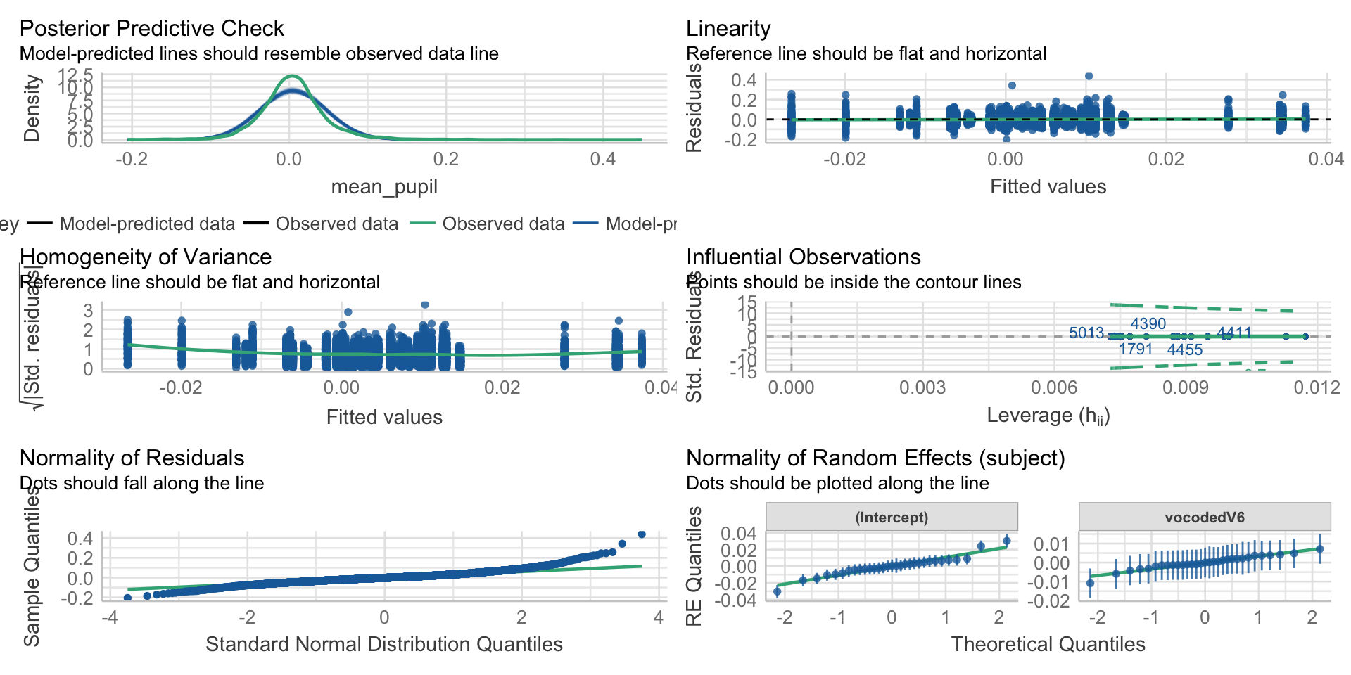
Fitting and Interpreting Models
Linear regression
Null model (unconditional means)
library(lme4) # pop linear modeling package

null_model <- lmer(mean_pupil ~ (1|subject), data = eye)

summary(null_model)
Linear mixed model fit by REML. t-tests use Satterthwaite's method [
lmerModLmerTest]
Formula: mean_pupil ~ (1 | subject)
Data: eye
REML criterion at convergence: -19811.6
Scaled residuals:
Min 1Q Median 3Q Max
-5.1411 -0.5530 -0.0463 0.4822 10.8130
Random effects:
Groups Name Variance Std.Dev.
subject (Intercept) 0.0001303 0.01142
Residual 0.0016840 0.04104
Number of obs: 5609, groups: subject, 31
Fixed effects:
Estimate Std. Error df t value Pr(>|t|)
(Intercept) 0.005227 0.002124 29.457784 2.461 0.0199 *
---
Signif. codes: 0 '***' 0.001 '**' 0.01 '*' 0.05 '.' 0.1 ' ' 1Intraclass correlation (ICC)
ICC is a standardized way of expressing how much variance is due to clustering/group
- Ranges from 0-1
Also, can be interpreted as correlation among observations within cluster/group
If ICC is sufficiently low (i.e., \(\rho\) < .1), then you don’t have to use MLM! BUT YOU PROBABLY SHOULD 🙂
Calculating ICC
Run baseline (null) model
Get intercept variance and residual variance
\[\mathrm{ICC}=\frac{\text { between-group variability }}{\text { between-group variability+within-group variability}}\]
\[ ICC=\frac{\operatorname{Var}\left(u_{0 j}\right)}{\operatorname{Var}\left(u_{0 j}\right)+\operatorname{Var}\left(r_{i j}\right)}=\frac{\tau_{00}}{\tau_{00}+\sigma^{2}} \]
Fixed effects
- Interpretation same as lm
# add the fixed effect of vocode
inter_model <- lmer(mean_pupil ~vocoded+(1|subject), data = eye)

#grab the fixed effects
broom.mixed::tidy(inter_model) %>% filter(effect == "fixed")| effect | group | term | estimate | std.error | statistic | df | p.value |
|---|---|---|---|---|---|---|---|
| fixed | (Intercept) | 0.00369 | 0.0022 | 1.68 | 33.6 | 0.102 | |
| fixed | vocodedV6 | 0.00306 | 0.0011 | 2.79 | 5.58e+03 | 0.00526 |
Default behavior is leave out *p*-values (Doug Bates doesn’t like them)
- Install `lmerTest` to include *p*-values
Random effects/variance components
Tells us how much variability there is around the fixed intercept/slope
How much does the average pupil size change between participants
Visualize random effects
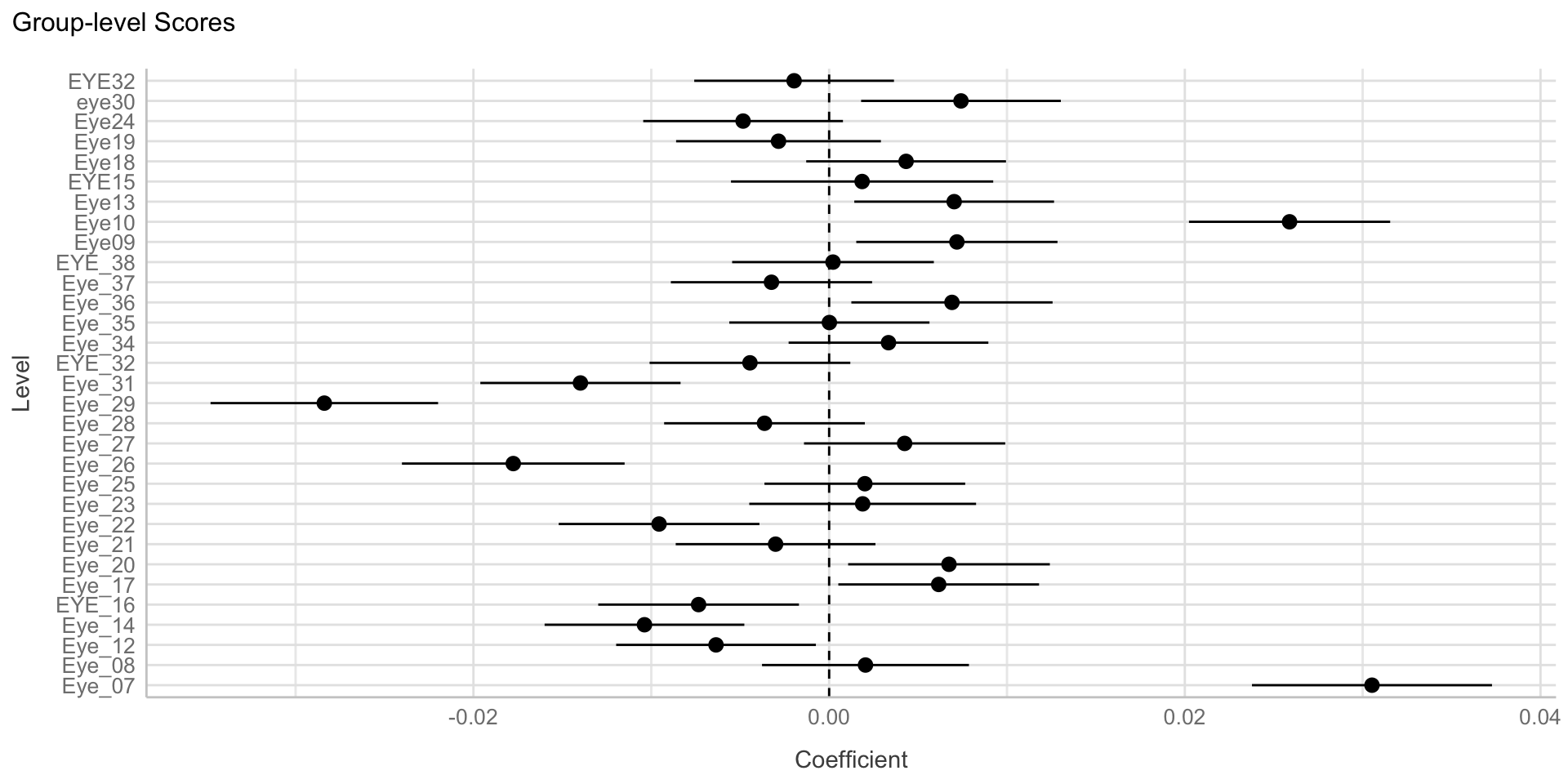
Maximal model: Fixed effect random intercepts (subject) and slopes (vocoded) model
| effect | group | term | estimate | std.error | statistic | df | p.value |
|---|---|---|---|---|---|---|---|
| fixed | (Intercept) | 0.00364 | 0.00223 | 1.63 | 28.9 | 0.114 | |
| fixed | vocodedV6 | 0.00312 | 0.00145 | 2.15 | 30.5 | 0.0396 | |
| ran_pars | subject | sd__(Intercept) | 0.0117 | ||||
| ran_pars | subject | cor__(Intercept).vocodedV6 | -0.195 | ||||
| ran_pars | subject | sd__vocodedV6 | 0.00531 | ||||
| ran_pars | Residual | sd__Observation | 0.0409 |
Using emmeans
- Get factor means and contrasts
 vocoded  emmean      SE  df asymp.LCL asymp.UCL
 NS      0.00364 0.00223 Inf -0.000737   0.00802
 V6      0.00677 0.00226 Inf  0.002334   0.01120

Degrees-of-freedom method: asymptotic
Confidence level used: 0.95 emmeans(max_model, specs = "vocoded") %>%
pairs() # use this to get pariwise compairsons between levels of factors contrast estimate SE df z.ratio p.value
NS - V6 -0.00312 0.00145 Inf -2.150 0.0316
Degrees-of-freedom method: asymptotic Maximal models
Keep it maximal1Whatever can vary, should vary
- include random slopes only if it is a within cluster manipulation
Only when there is convergence issues should you remove terms
Decreases Type 1 error
Visualize random intercepts + slopes
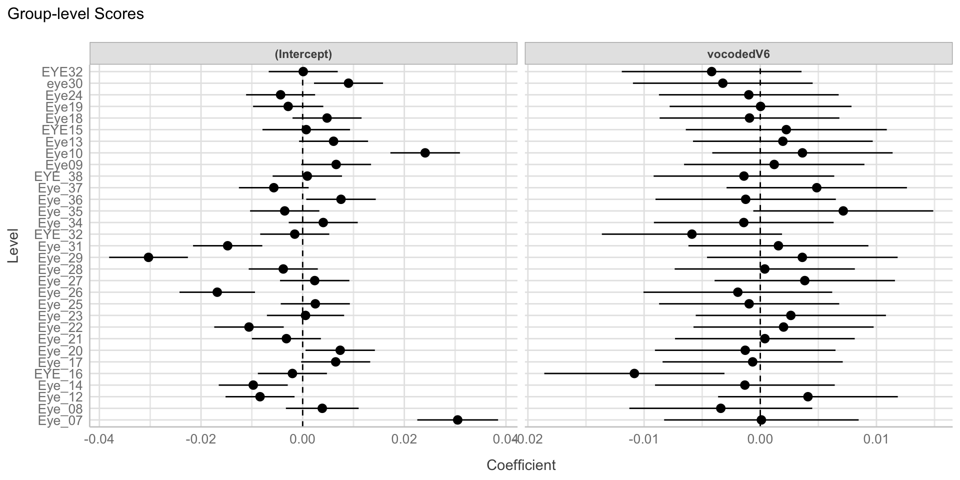
Random effects/variance components
Correlation between random intercepts and slopes
Negative correlation
- Higher intercept (for normal speech) less of effect (lower slope)
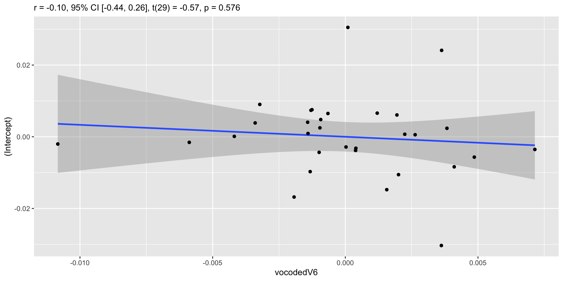
Model comparison
Can compare models using
anovafunction ortest_likelihoodratiofromeasystats- Will be refit using ML
LRT
For more complex models, use LRT chi-square (drop-in deviance test)
- Can be interpreted as main effects and interactions
- Use
afex
Visualization
Easystats
- Easily visualize data
pupil_data_mean <- eye %>%
  group_by(subject, vocoded) %>%
  summarise(mean_pup=mean(mean_pupil, na.rm=TRUE)) %>%
  ungroup()

mod_plot <- max_model %>%
  estimate_means("vocoded") %>%
  as.data.frame()

pupil_plot_lmer <- ggplot(pupil_data_mean, aes(x = vocoded, y = mean_pup)) +
  geom_violinhalf(aes(fill = vocoded), color = "white") +
  geom_jitter2(width = 0.05, alpha = 0.5, size=5) +  # Add pointrange and line from means
  geom_line(aes(y=mean_pup, group=subject))+
  geom_line(data = mod_plot, aes(y = Mean, group = 1), size = 3) +
  geom_pointrange(
    data = mod_plot,
    aes(y = Mean, ymin = CI_low, ymax = CI_high),
    size = 2,
    color = "green"
  ) +
  # Improve colors
  scale_fill_material() +
  theme_modern() +
  ggtitle("Pupil Effect", subtitle = "White dots represent model mean and error bars represent 95% CIs. Black dots are group level means for each person")
Easystats
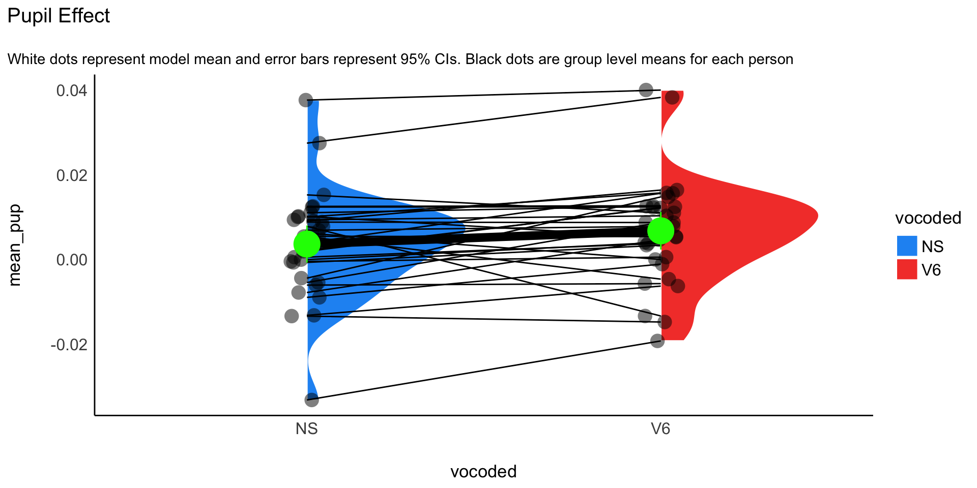
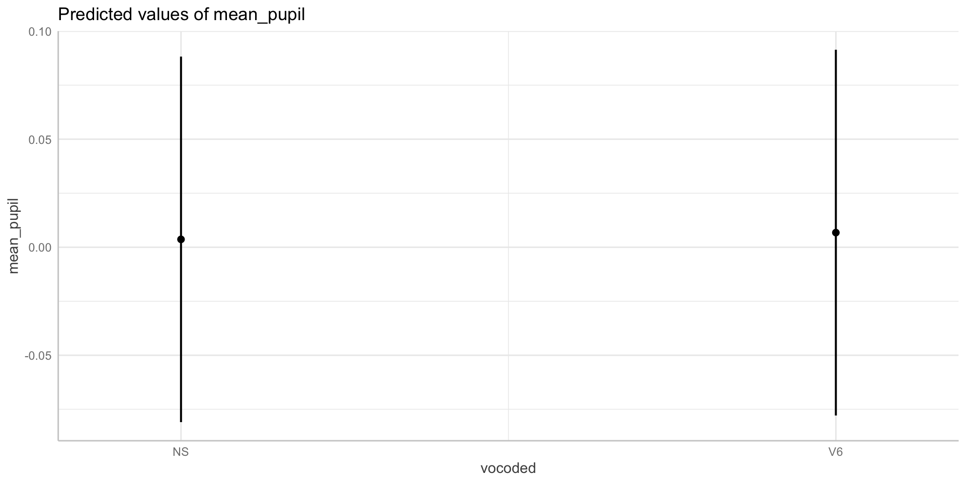
ggeffects
Effect size
Highly debated
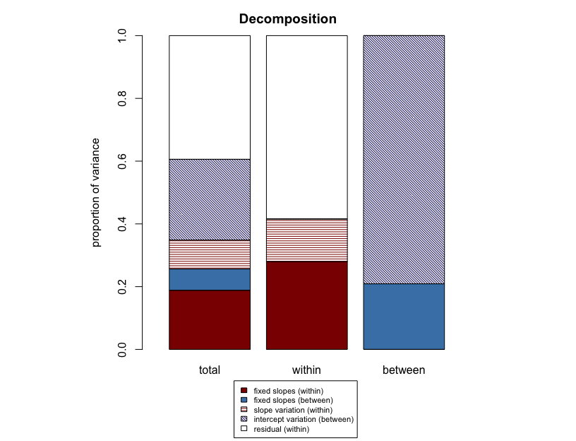
- Report pseudo-\(R^2\) for marginal (fixed) and conditional model (random) parts
Transform f to \(\eta_p^2\) (when using afex::mixed)
r2mlm
Write-up
We fitted a linear mixed model (estimated using REML and nloptwrap optimizer)
to predict mean_pupil with vocoded (formula: mean_pupil ~ vocoded). The model
included vocoded as random effects (formula: ~1 + vocoded | subject). The
model's total explanatory power is weak (conditional R2 = 0.08) and the part
related to the fixed effects alone (marginal R2) is of 1.34e-03. The model's
intercept, corresponding to vocoded = NS, is at 3.64e-03 (95% CI [-7.38e-04,
8.02e-03], t(5603) = 1.63, p = 0.103). Within this model:

  - The effect of vocoded [V6] is statistically significant and positive (beta =
3.12e-03, 95% CI [2.75e-04, 5.97e-03], t(5603) = 2.15, p = 0.032; Std. beta =
0.07, 95% CI [6.49e-03, 0.14])

Standardized parameters were obtained by fitting the model on a standardized
version of the dataset. 95% Confidence Intervals (CIs) and p-values were
computed using a Wald t-distribution approximation.
Table
| (1) | |
|---|---|
| (Intercept) | 0.004 |
| (0.002) | |
| vocodedV6 | 0.003 |
| (0.001) | |
| SD (Intercept subject) | 0.012 |
| SD (vocodedV6 subject) | 0.005 |
| Cor (Intercept~vocodedV6 subject) | −0.195 |
| SD (Observations) | 0.041 |
| Num.Obs. | 5609 |
| R2 Marg. | 0.001 |
| R2 Cond. | 0.077 |
| AIC | −19801.7 |
| BIC | −19761.9 |
| ICC | 0.1 |
| RMSE | 0.04 |
Generalized linear mixed models
We can fit most of the models we talked about this semester as a multilevel model
Easy to fit Bayesian equivalents as well (using
brms)
Shrinkage
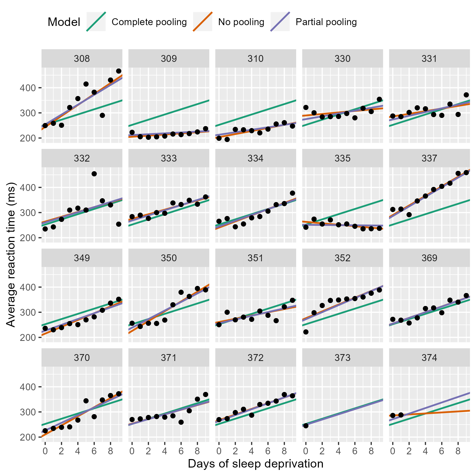
(https://www.tjmahr.com/plotting-partial-pooling-in-mixed-effects-models/)
Centering
You must ensure that the zero value for each predictor is meaningful before running the model
Categorical variables:
- Effect-coding or contrast-coding
Continuous Predictors:
In MLM, there are two ways to center, by the grand mean or the group mean
Group- vs. grand-mean centering
Grand-mean centering: \(x_{i} - x\)
- Variable represents each observation’s deviation from everyone’s norm, regardless of group
Group-mean centering: \(x_{ij} - x_j\)
- Variable represents each observation’s deviation from their group’s norm
Group- vs. grand-mean centering
Level 1 predictors
Grand-mean center
- Include means of level 2
- Allows us to directly test within-group effect
Group-mean center
- Level 1 coefficient will always be with within-group effect, regardless of whether the group means are included at Level 2 or not
- If level 2 means included, coefficient represents the between-groups effect
Group mean center in R
library(datawizard) #easystats

# how to group mean center
d <- d %>%
  # Grand mean centering (CMC)
  mutate(iv.gmc = iv-mean(iv)) %>%
  # Person mean centering (more generally, centering within cluster)
  group_by(id) %>%
  mutate(iv.cm = mean(iv),
         iv.cwc = iv-iv.cm) %>%
  ungroup %>%
  # Grand mean centering of the aggregated variable
  mutate(iv.cmc = iv.cm-mean(iv.cm))
# data wizard way
x <- demean(x, select=c("x"), group="ID") #gets within-group cluster
PSY 504: Advanced Statistics
